Topics in High-Performance Messaging
-by-
Robert A. Van Valzah
Todd L. Montgomery
Eric Bowden
Copyright © 2004 - 2023 Informatica, LLC.
July 2023
Abstract
The Informatica Ultra Messaging team has worked together in the field of high-performance messaging for many years, and in that time, have seen some messaging systems that worked well and some that didn't. Successful deployment of a messaging system requires background information that is not easily available; most of what we know, we had to learn in the school of hard knocks. To save others a knock or two, we have collected here the essential background information and commentary on some of the issues involved in successful deployments. This information is organized as a series of topics around which there seems to be confusion or uncertainty.
Please contact us if you have questions or comments.
1. Introduction
In the field of high-performance messaging systems, performance tends to be the dominant factor in making design decisions. In this context, "performance" can indicate high message rates, high payload data transfer rates, low latency, high scalability, high efficiency, or all of the above. Such factors tend to be important in applications like financial market data, satellite, telemetry, and military command & control.
Successful deployment of high-performance messaging systems requires cross-disciplinary knowledge. System-level issues must be considered including network, OS, and host hardware issues.
In this document, we frequently refer to our Ultra Messaging ("UM") product, but we believe that the concepts presented are applicable to a wide variety of high-performance networking applications. If you are interested in learning more about UM, contact us at dlmessagingsuptcc@informatica.com.
2. TCP Latency
TCP can be used for latency-sensitive applications, but several factors must be considered when choosing it over other protocols that may be better suited to latency-sensitive applications.
TCP provides low-latency delivery only if:
-
All receivers can always keep up with the sender
-
The network is never congested
This essentially boils down to "TCP is OK for latency-sensitive applications if nothing ever goes wrong."
A little historical perspective helps in understanding TCP. It's easy for one user of a network to think about TCP only from the point of view of someone who needs to reliably transfer data though the network. But network architects and administrators often have other goals. They want to make sure that all users of a network can share the available bandwidth equally and to assure that the network is always available. If TCP allowed all users to send data whenever they wanted, bandwidth would not be shared equally and network throughput might collapse in response to the load. Hence the focus of TCP is deciding when to allow a user to send data. The protocol architects who created TCP named it Transmission Control Protocol to reflect this focus. Said differently, TCP adds latency whenever necessary to maintain equal bandwidth sharing and network stability. Latency-sensitive applications typically don't want a transport protocol deciding when they can send.
2.1. TCP Latency Behavior
Broadly speaking, the way that TCP does rate control makes it unsuitable for latency-sensitive applications. (See Section 3 for a contrast with other ways of doing rate control.) A TCP receiver will add latency whenever packet loss or network routing causes packets to arrive out of order. A TCP sender will add latency when going faster would cause network congestion or when it would be sending faster than the receiver can process the incoming data.
2.2. TCP Receiver-Side Latency
TCP only supports one delivery model: in-order delivery. This means that a TCP receiver must add latency whenever data arrives out of order so as to put the data back in order. TCP also often unnecessarily retransmits data that was already successfully received after out-of-order data is received.
There are two main causes of out-of-order data reception. The most frequent cause is packet loss, either at the physical or network-layer. Another, less frequent cause of out-of-order data reception is that packets can take different paths through the network; one path have more latency than another. In either case, TCP inserts latency to put the packets back in order, as illustrated in Figure 1.

Note that the receiving application cannot receive packet 3 until (the retransmitted) packet 2 has arrived. The receiving TCP stack adds latency while waiting for the successful arrival of packet 2 before packet 3 can be delivered.
Contrast this with the case where a transport with an arrival-order delivery model is used as shown in Figure 2.

Note that packet 3 is delivered to the application layer as soon as it arrives.
TCP cannot provide arrival order delivery, but UDP can. However, simple UDP is awkward for many applications because it provides no reliability in delivery. In the above example, it becomes the application's responsibility to detect packet 2's loss and request its retransmission.
With this in mind, we created a reliable multicast protocol called LBT-RM. It offers lower latency than TCP since it uses UDP and arrival order delivery, but it can also provide reliability through the built-in loss detection and retransmission logic. Of course, each message delivered by LBT-RM has a sequence number so that the application has message sequencing information available if needed.
If you're curious about how much latency is being added by the TCP in-order delivery model, you can often get a hint by looking at output from the netstat -s command. Look for statistics from TCP. In particular, look for out-of-order packets received and total packets received. Divide these two numbers to get a percentage of packets that are being delayed by TCP in-order delivery.
For example, consider this output from netstat -s.
tcp:
. . .
      2854 packets received
. . .
          172 out-of-order packets (151915 bytes)
The above example statistics show that about 6% of all incoming TCP packets are being delayed due the requirement of in-order delivery (this is pretty high; we hope that you are not experiencing this degree of packet loss). Be aware that netstat output tends to vary quite a bit from operating system to operating system, so your output may look quite different from the above.
2.3. TCP Sender-Side Latency
TCP is designed to send as fast as possible while maintaining equal bandwidth sharing with all other TCP streams and reliable delivery. A TCP sender may slow down for two reasons:
-
Going faster would cause network congestion.
-
Going faster would send data faster than the receiver can process it.
If you were to liken TCP to an automobile driver, you'd have to call TCP the most lead-footed yet considerate driver on the road. As long as the road ahead is clear, TCP will drive as fast as possible. But as soon as other traffic appears on the road, TCP will slow down so that other drivers (i.e. other TCP streams) have a equal shot at using the road too. The technical term for this behavior is congestion control. When a network becomes congested, the TCP algorithms insure that the pain is felt equally by all active TCP streams, which is exactly the behavior you want if your primary concern is bandwidth sharing and network stability. However, if you have a latency-sensitive application, you would prefer that it get priority, leaving the other less-critical applications to divide up the remaining bandwidth. That is, you would like to be able to add flashing lights and a siren to your latency-sensitive applications.
It's important to note that TCP uses two different mechanisms to measure congestion: round-trip time (RTT) and packet loss. (See Myth: All Packet Loss is Bad for details.) Sticking with the automobile analogy, an increase in RTT causes TCP to take its foot off the gas to coast while packet loss causes it to step on the brakes. TCP cuts its transmission rate by 1/2 every time it detects loss. This can add additional latency after the original loss. Even small amounts of loss can drastically cut TCP throughput.
TCP also makes sure that the sender does not send data faster than the receiver can process it. A certain amount of buffer space is allocated on the receiver, and when that buffer fills, the sender is blocked from sending more. The technical term for this behavior is flow control. TCP's philosophy is "better late than never". Many latency-sensitive applications prefer the "better never than late" philosophy. At the very least, a slow, possibly problematic receiver should not cause unnecessary latency with other receivers. Obviously, there needs to be enough buffer space to handle normal periods of traffic bursts and temporary receiver slow-downs, but if/when those buffers do fill up, it's better to drop data than block the sender.
2.4. TCP Latency Recommendations
It's probably best to avoid using TCP for latency-sensitive applications. As an alternative, consider protocols that slow down a sender only when required for network stability. For example, the Ultra Messaging product offers protocols like LBT-RM that have been designed specifically for latency-sensitive applications. Such protocols allow reliable yet latency-bounded delivery without sacrificing network stability.
When TCP cannot be avoided, it's probably best to:
-
Use clever buffering and non-blocking sockets with TCP to drop data for congested TCP connections when data loss is preferable over latency. Ultra Messaging uses such buffering for its source-paced TCP feature.
-
Consider disabling Nagle's algorithm with the
TCP_NODELAYoption tosetsockopt(). Although this may produce decreased latency, it often does so at the expense of efficiency. -
Route latency-sensitive TCP traffic over a dedicated network where congestion is minimized or eliminated.
-
Keep kernel socket buffers to a minimum so that latency is not added as data is stored in such buffers. TCP windows substantially larger than the bandwidth-delay product (BDP) for the network will not increase TCP throughput but they can add latency.
3. Group Rate Control
Any application seeking to deliver the same data stream to a group of receivers faces challenges in dealing with slow receivers. Group members that can keep up with the sender may be inconvenienced or perhaps even harmed by those that can't keep up. At the very least, slow receivers cause the sender to use memory for buffering that could perhaps be put to other uses. Buffering adds latency, at least for the slow receiver and perhaps for all receivers. Note that rate control issues are present for groups using either multicast or unicast addressing.
3.1. The Crybaby Receiver Problem
Often, the whole group suffers due to the problems of one member. In extreme cases, the throughput for the group falls to zero because resources that the group shares are dedicated to the needs of one or a few members. Examples of shared resources include the sender's CPU, memory, and network bandwidth. This phenomenon is sometimes called the "crybaby receiver problem" because the cries (e.g. retransmission requests) from one receiver dominate the attention of the parent (the sender).
The chance of encountering a crybaby receiver problem increases as the number of receivers in the group increases. Odds are that at least one receiver will be having difficulty keeping up if the group is large enough.
As long as all receivers in the group are best served by the sender running at the same speed, there is no conflict within the group. Scenarios such as crybaby receivers often present a conflict between what's best for a few members and what's best for the majority. Robust systems will have policies for dealing with the apparent conflict and consistently resolving it.
3.2. Group Rate Control Policies
There are three rate control policies that a sender can use for dealing with such conflict within a group. Two are extremes and the third is a middle ground.
3.2.1. Policy Extreme 1
The sender slows down to the rate of the slowest receiver. If the sender cannot control the rate at which new data arrives for transmission to the group, it must either buffer the data until the slowest receiver is ready or drop it. All receivers in the group then experience latency or lost data.
3.2.2. Policy Extreme 2
The sender sends as fast as is convenient for it. This is often the rate at which new data arrives or is generated. It is often possible that this rate is too fast for even the fastest receivers. All receivers that can't keep up with the rate most convenient for the sender will experience lost data. This is often called "uncontrolled" since there is no mechanism to regulate the rate used by the sender.
3.2.3. Middle Ground
The sender operates within a set of boundaries established a system administrator or architect. The sender's goal is to minimize data loss and latency in the receiver group while staying within the configured limits.
3.3. Group Rate Control Consequences
The extreme policies have potentially dire consequences for many applications. For example, neither is ideal for market data and other types of latency-sensitive data.
Extreme 2 is the policy most often used. Successful use of it requires that networks and receivers be provisioned to keep up with the fastest rate that might be convenient for the sender. Such policies often leave little bandwidth for TCP traffic and can be vulnerable to "NAK storms" and other maladies which can destabilize the entire network.
Extreme 1 is appropriate only for transactional applications where it's more important for the group to stay in sync than for the group to have low latency.
The middle ground policy is ideal for many latency-sensitive applications such as transport of financial market data. It allows for low-latency reliable delivery while maintaining the stability of the network. No amount of overload can cause a "NAK storm" or other network outage when the policy is established with knowledge of the capabilities of the network.
3.4. Policy Selection
The need to establish a group rate control policy is often not apparent to those accustomed to dealing with two-party communication (e.g. TCP). When there are only two parties communicating, one policy is commonly used: the sender goes as fast as it can without going faster than the receiver or being unfair to others on the network. (See Section 2 for details.) This is the only sensible policy for applications that can withstand some latency and cannot withstand data loss. With two-party communication using TCP, it's the only policy choice you have. However, group communication with one sender and many receivers opens up all of the policy possibilities mentioned above.
Some messaging systems support only one policy and hence require no policy configuration. Others may allow a choice of policy. Any middle ground policy will need to be configured to establish the boundaries within which it should operate.
The best results are obtained when the specific needs of a messaging application have been considered and the messaging system has been configured to reflect them. A messaging system has no means to automatically select from among the available group rate control policies. Human judgment is required.
3.5. Group Rate Control Recommendations
A group rate control policy should be chosen to match the needs of the application serving the group. The choice is often made by weighing the benefits of low latency against reliable delivery. These benefits have to be considered for individuals within the group and for the group as a whole.
In some applications, members of the group benefit from the presence of other members. In these applications, the group benefit from reliable reception among all receivers may outweigh the pain of added latency or limited group throughput. Consider a group of servers that share the load from a common set of clients. Assume that the servers have to stay synchronized with a stream of messages to be able to answer client queries. If one server leaves the group because it lost some messages, the clients it was serving would move to the remaining servers. This could lead to a domino effect where a traffic burst caused the slowest server to drop from the group which in turn increased the load on the other servers causing them to fail in turn as well. Clearly in a situation like this, it's better for the whole group of servers to slow down a bit during a traffic peak so that even the slowest among them can keep up without loss. The appropriate group rate control policy for such an application is Extreme 1 (see Section 3.2.1).
Other applications see no incremental benefit for the group if all members experience reliable reception. Consider a group of independent traders who all subscribe to a market data stream. Traders who can keep up with the rate convenient for the sender do not want the sender to slow down for those who can't. Extreme 2 (see Section 3.2.2) is probably the appropriate policy for an application like this. However, care must be taken to prevent the sender from going faster than even the fastest trader as that often leads to NAK storms from which there is no recovery.
The Ultra Messaging team recommends a careful analysis of the policies that are best for the group using an application and for individual members of the group. The rate control policy best suited to your application will generally emerge from such an analysis. We have found that it is possible to build stable, low-latency messaging systems with careful network design and a messaging layer like Ultra Messaging that supports a middle ground policy through the use of rate controls.
3.6. Group Rate Control and Transport Protocols
Once you've chosen a group rate control policy appropriate for your application, it's important to chose a transport protocol that can implement your chosen policy. Some transport protocols offer only the extreme policies while others allow parameters to be set to implement a middle ground policy.
UDP provides no rate control at all, so it follows group policy Extreme 2 above (see Section 3.2.2).
TCP doesn't operate naturally as a group communication protocol since it only supports unicast addressing. However, when TCP is used to send copies of the same data stream to more than one receiver, all of the group rate control issues discussed above are present. TCP's inherent flow control feature follows group policy Extreme 1 described above (see Section 3.2.1). If the sender is willing to use non-blocking I/O and manage buffering, then Extreme 2 and middle ground policies can be implemented to some degree.
Some reliable multicast transport protocols provide no rate control at all (e.g. TIBCO Rendezvous), some provide only a fixed maximum rate limit (e.g. PGM), and some provide separate rate controls for initial data transmission and retransmission (e.g. LBT-RM from Ultra Messaging). See Section 15 for details.
4. Ethernet Flow Control
In the process of testing the LBT-RM reliable multicast protocol used in the Ultra Messaging product, we noticed that some Ethernet switches and NICs now implement a form of flow control that can cause unexpected results. This is commonly seen in mixed speed networks (e.g. 10/100 Mbps or 100/1000 Mbps). We have seen apparently strange results such as two machines being able to send TCP at 100 Mbps but being limited to 10 Mbps for multicast using LBT-RM.
The cause of this seems to be Ethernet switches and NICs that implement the IEEE 802.3x Ethernet flow control standard. It seems to be most commonly implemented in desktop-grade switches. Infrastructure-grade equipment makers seem to have identified the potential harm that Ethernet flow control can cause and decided to implement it carefully if at all.
The intent of Ethernet flow control is to prevent loss in switches by providing back pressure to the sending NIC on ports that are going too fast to avoid loss. While this sounds like a good idea on the surface, higher-layer protocols like TCP were designed to rely on loss as a signal that they should send more slowly. Hence, at the very least, Ethernet flow control duplicates the flow control mechanism already built into TCP. At worst, it unnecessarily slows senders when there's no need.
Problems can happen with multicast on mixed-speed networks if a switch with Ethernet flow control applies back pressure on a multicast sender when it tries to go faster than the slowest active port on the switch. Consider the scenario where two machines X and Y are connected to a switch at 100 Mbps while a third machine Z is connected to the same switch at 10 Mbps. X can send TCP traffic to Y at 100 Mbps since the switch sees no congestion delivering data to Y's switch port. But if X starts sending multicast, the switch tries to forward the multicast to Z's switch port as well as to Y's. Since Z is limited to 10 Mbps, the switch senses congestion and prevents X from sending faster than 10 Mbps.
We have tested switches that behave this way even if there are no multicast receivers on the slow ports. That is, these switches did not have an IGMP snooping feature or an equivalent that would prevent multicast traffic from being forwarded out ports where there were no interested receivers. It seems best to avoid such switches when using LBT-RM. Any production system with switches like this may be vulnerable to the problem where the network runs fine until one day somebody plugs an old laptop into a conference room jack and inadvertently limits all the multicast sources to 10 Mbps.
It may also be possible to configure hosts to ignore flow control signals from switches. For example, on Linux, the /sbin/ethtool command may be able to configure a host to ignore pause signals that are sent from a switch sensing congestion. Module configuration parameters or registry settings might also be appropriate.
5. Packet Loss Myths
Packet loss is a common occurrence that is often misunderstood. Many applications can run successfully with little or no attention paid to packet loss. However, latency-sensitive applications can often benefit from improved performance if packet loss is better understood. We have encountered many myths surrounding packet loss in our Ultra Messaging development. The following paragraphs address these myths and provide links to additional helpful information.
- Myth--Most loss is caused by transmission errors, gamma rays, etc.
- Myth--There is no loss in networks that are operating properly.
- Myth--Loss only happens in networks (i.e. not in hosts).
- Myth--All packet loss is bad.
- Myth--Unicast and multicast loss always go together.
Reality--Our experience and anecdotal evidence from others indicates that buffer overflow is the most common cause of packet loss. These buffers may be in network hardware (e.g. switches and routers) or it may be in operating systems. See Section 7 for background information.
Reality--The normal operation of TCP congestion control may cause loss due to queue overflow. See this report for more information. Loss rates of several percent were common under heavy congestion.
Reality--The flow control mechanism of TCP should prevent packet loss due to host buffer overflows. However, UDP contains no flow-control mechanism leaving the possibility that UDP receiver buffers will overflow. Hosts receiving high-volume UDP traffic often experience internal packet loss due to UDP buffer overflow. See Section 7.6 for more on the contrast between TCP buffering and UDP buffering. See Section 8.9 for advice on detecting UDP buffer overflow in a host.
Reality--Packet loss plays at least two important, beneficial roles:
-
Implicit signaling of congestion: TCP uses loss to discover contention with other TCP streams. Each TCP stream passing through a congestion point must dynamically discover the existence of other streams sharing the congestion point in order to fairly share the available bandwidth. They do this by monitoring 1) the SRTT (Smoothed Round-Trip Time) as an indication of queue depth, and 2) packet loss as an indication of queue overflow. Hence TCP relies upon packet loss as an implicit signal of network congestion. See Section 2.3 for discussion of the impact this can have on latency.
-
Efficient discarding of stale, latency-sensitive data: See Section 8.1 for more information.
6. Monitoring Messaging Systems
Production deployments of messaging systems often employ real-time monitoring and rapid human intervention if something goes wrong. Urgent reaction to problems detected by real-time monitoring can be required to prevent the messaging system from becoming unstable. A common example of this is using real-time monitoring to discover crybaby receivers and repair or remove them from the network. (See Section 3.1 for details.) The presence of a crybaby receiver can starve lossless receivers of bandwidth needed for new messages in what is commonly called a NAK storm.
Ultra Messaging is designed so that real-time monitoring and urgent response are not required. The design of UM encourages stable operation by allowing you to pre-configure how UM will use resources under all traffic and network conditions. Hence manual intervention is not required when those conditions occur.
Monitoring UM still fills important roles other than maintaining stable operation. Chiefly among these are capacity planning and gaining a better understanding the latency that UM adds to recover from loss. Collecting accumulated statistics from all sources and all receivers once per day is generally adequate for these purposes.
7. UDP Buffering Background
Understanding UDP buffering is critical to leveraging the maximum possible performance from the reliable multicast (LBT-RM) and reliable unicast (LBT-RU) protocols within the Ultra Messaging product. Our reliable unicast and reliable multicast protocols use UDP to achieve control of transport latency that would be impossible with TCP.
Much of what we've learned deploying our UDP-based protocols should be applicable to other high-performance work with UDP. We have collected here some of the background information that we've found helpful in understanding issues related to UDP buffering.
Although UDP is buffered on both the send and receive side, we've seldom seen a need to be concerned with send-side UDP buffering. For brevity, we'll use simply "UDP buffering" to refer to receive-side UDP buffering.
7.1. Function of UDP Buffering
UDP packets may arrive in bursts because they were sent rapidly or because they were bunched together by the normal buffering action of network switches and routers.
Similarly, UDP packets may be consumed rapidly when CPU time is available to run the consuming application. Or they may be consumed slowly because CPU time is being used to run other processes.
UDP receive buffering serves to match the arrival rate of UDP packets (or "datagrams") with their consumption rate by an application program. Of course, buffering cannot help cases where the long-term average send rate exceeds the average receive rate.
7.2. Importance of UDP Buffering
UDP receive buffering is done in the operating system kernel. Typically the kernel allocates a fixed-size buffer for each socket receiving UDP. Buffer space is consumed for every UDP packet that has arrived but has not yet been delivered to the consuming application. Unused space is generally unavailable for other purposes because it must be readily available for the possible arrival of more packets. See Section 7.4 for a further explanation.
If a UDP packet arrives for a socket with a full buffer, it is discarded by the kernel and a counter is incremented. See Section 8.9 for information on detecting UDP loss. A common myth is that all UDP loss is bad. (See Myth: All Packet Loss is Bad.) Even if it's not all bad, UDP loss does have its consequences. (See Section 8.3.)
7.3. Kernel and User Mode Roles in UDP Buffering
The memory required for the kernel to do UDP buffering is a scarce resource that the kernel tries to allocate wisely. (See Section 7.4 for more on the rationale.) Applications expecting low-volume UDP traffic or those expecting low CPU scheduling latency (see Section 17.6) need not consume very much of this scarce resource. Applications expecting high-volume UDP traffic or those expecting a high CPU scheduling latency may be justified in consuming more UDP buffer space than others.
Typically, the kernel allocates a modest-size buffer when a UDP socket is created.
This is generally adequate for less-demanding applications. Applications requiring a
larger UDP receive buffer can request it with the system call setsockopt(...SO_RCVBUF...).
Explicit configuration of the application may be required before it will request a
larger UDP buffer. (For UM, this is the context option transport_lbtrm_receiver_socket_buffer.)
The kernel configuration will allow such requests to succeed only up to a set size limit. This limit may often be increased by changing the kernel configuration. See Section 8.8 for information on setting kernel UDP buffer limits.
Hence two steps are often required to get adequate UDP buffer space:
-
Change the kernel configuration to increase the limit on the largest UDP buffer allocation that it will allow.
-
Change the application to request a larger UDP buffer.
7.4. Unix Kernel UDP Buffer Limit Rationale
It may seem to some that the default maximum UDP buffer size on many Unix kernels is a bit stingy. Understanding the rationale behind these limits may help.
UDP is typically used for low-volume query/response work (e.g. DNS, NTP, etc.). The kernel default limits assume that UDP will be used in this way.
UDP kernel buffer space is allocated from physical memory for the exclusive use of one process. The kernel tries to make sure that one process can't starve others for physical memory by allocating large UDP buffers that exhaust all the physical memory on a machine.
To some degree, the meager default limits are a legacy from the days when 4 MB was a lot of physical memory. In these days when several gigabytes of physical memory space is common, such small default limits seem particularly stingy.
7.5. UDP Buffering and CPU Scheduling Latency
For the lowest-possible latency, the operating system would run a process wishing to receive a UDP packet as soon as the packet arrives. In practice, the operating system may allow other processes to finish using their CPU time slice first. It may also seek to improve efficiency by accumulating several UDP packets before running the application. We will call the time that elapses between when a UDP packet arrives and when the consuming application gets to run on a CPU the CPU scheduling latency. See Section 17.6 for more information. UDP buffer space fills during CPU scheduling latency and empties when the consuming process runs on a CPU. CPU scheduling latency plays a key role optimal UDP buffer sizing. See Section 8.1 for more information.
7.6. TCP Receive Buffering vs. UDP Receive Buffering
The operating system kernel automatically allocates TCP receive buffer space based on policy settings, available memory, and other factors. TCP in the sending kernel continuously monitors available receive buffer space in the receiving kernel. When a TCP receive buffer fills up, the sending kernel prevents the sending application from using CPU time to generate any more data for the connection. This behavior is called "flow control." In a nutshell, it prevents the receiver buffer space from overflowing by adding latency at the sender. We say that the speed of a TCP sender is "receiver-paced" because the sending application is prevented from sending when data cannot be delivered to the receiving application.
The OS kernel also allocates UDP receive buffer space based on policy settings. However, UDP senders do not monitor available UDP receive buffer space in the receiving kernel. UDP receivers simply discard incoming packets once all available buffer space is exhausted. We say that the speed of a UDP sender is "sender-paced" because the sending application can send whenever it wants without regard to available buffer space in the receiving kernel.
The default TCP buffer settings are generally adequate and usually require adjustment only for unusual network parameters or performance goals.
The appropriate size for an application's UDP receive buffer is influenced by factors that cannot be known when operating system default policies are established. Further, there is nothing the operating system can do to automatically discover the appropriate size. An application may know that it would benefit from a UDP receive buffer larger or smaller than the default used by the operating system. It can request a non-default UDP buffer size from the operating system, but the request may not be granted due to a policy limit. See Section 7.4 for reasons behind such policy limits. Operating system policies may have to be adjusted to successfully run high-performance UDP applications like UM. See Section 8.8 to change operating system policies.
8. UDP Buffer Sizing
There are many questions surrounding UDP buffer sizing. What is the optimal size? What are the consequences of an improperly sized UDP buffer? What are the equations needed to compute an appropriate size for a UDP buffer? What default limit will the OS kernel place on UDP buffer size and how can I change it? How can I tell if I'm having UDP loss problems due to buffers that are too small? Answers to these questions and more are given in the following sections.
8.1. Optimal UDP Buffer Sizing
UDP buffer sizes should be large enough to allow an application to endure the normal variance in CPU scheduling latency without suffering packet loss. They should also be small enough to prevent the application from having to read through excessively old data following an unusual spike in CPU scheduling latency.
8.2. UDP Buffer Space Too Small: Consequences
Too little UDP buffer space causes the operating system kernel to discard UDP packets. The resulting packet loss has consequences described below.
The kernel often keeps counts of UDP packets received and lost. See Section 8.9 for information on detecting UDP loss due to UDP buffer space overflow. A common myth is that all UDP loss is bad (see Myth: All Packet Loss is Bad).
8.3. UDP Loss: Consequences
In most cases, it's the secondary effects of UDP loss that matter most. That is, it's the reaction to the loss that has material consequences more so than the loss itself. Note that the consequences discussed here are independent of the cause of the loss. Inadequate UDP receive buffering is just one of the more common causes we've encountered deploying UM.
Consider these areas when assessing the consequences of UDP loss:
-
Latency--The time that passes between the initial transmission of a UDP packet and the eventual successful reception of a retransmission is latency that could have been avoided were it not for the intervening loss.
-
Bandwidth--UDP loss usually results in requests for retransmission, unless more up-to-date information is expected soon (e.g. in the case of stock quote updates). Bandwidth used for retransmissions may become significant, especially in cases where there is a large amount of loss or a large number of receivers experiencing loss. See Section 15 for more information on multicast retransmissions.
-
CPU Time--UDP loss causes the receiver to use CPU time to detect the loss, request one or more retransmissions, and perform the repair. Note that efficiently dealing with loss among a group of receivers requires the use of many timers, often of short-duration. Scheduling and processing such timers generally requires CPU time in both the operating system kernel ("system time") and in the application receiving UDP ("user time"). Additional CPU time is required to switch between kernel and user modes.
On the sender, CPU time is used to process retransmission requests and to send retransmissions as appropriate. As on the receiver, many timers are required for efficient retransmission processing, thus requiring many switches between kernel and user modes.
-
Memory--UDP receivers that can only process data in the order that it was initially sent must allocate memory while waiting for retransmissions to arrive. UDP loss causes such receivers to receive data in an order different than that used by the sender. Memory is used to restore the order in which it was initially sent.
Even UDP receivers that can process UDP packets in the order they arrive may not be able to tolerate duplication of packets. Such receivers must allocate memory to track which packets have been successfully processed and which have not.
UDP senders interested in reliable reception by their receivers must allocate memory to retain UDP packets after their initial transmission. Retained packets are used to fill retransmission requests.
8.4. UDP Buffer Space Too Large: Consequences
Even though too little UDP buffer space is definitely bad and more is generally better, it is still possible to have too much of a good thing. Perhaps the two most significant consequences of too much UDP buffer space are slower recovery from loss and physical memory usage. Each of these is discussed in turn below.
-
Slower Recovery--To best understand the consequences of too much UDP buffer space, consider a stream of packets that regularly updates the current value of a rapidly-changing variable in every tenth packet. Why buffer more than ten packets? Doing so would only increase the number of stale packets that must be discarded at the application layer. Given a data stream like this, it's generally better to configure a ten-packet buffer in the kernel so that no more than ten stale packets have to be read by the application before a return to fresh ones from the stream.
It's often counter-intuitive, but excessive UDP buffering can actually increase the recovery time following a large packet loss event. UDP receive buffers should be sized to match the latency budget allocated for CPU scheduling latency with knowledge of expected data rates. See Section 16 for more information on latency budgets. See Section 8.6 for a UDP buffer sizing equation.
-
Physical Memory Usage--It is possible to exhaust available physical memory with UDP buffer space. Requesting a UDP receive buffer of 32 MB and then invoking ten receiver applications uses 320 MB of physical memory. See Section 7.4 for more information.
8.5. UDP Buffer Size Equations: Latency
Assuming that an average rate is known for a UDP data stream, the amount of latency that would be added by a full UDP receive buffer can be computed as:
Max Latency = Buffer Size / Average Rate
Note: Take care to watch for different units in buffer size and average rate (e.g. kilobytes vs. megabits per second).
8.6. UDP Buffer Size Equations: Buffer Size
Assuming that an average rate is known for a UDP data stream, the buffer size needed to avoid loss a given worst case CPU scheduling latency can be computed as:
Buffer Size = Max Latency * Average Rate
Note: Since data rates are often measured in bits per second while buffers are often allocated in bytes, careful conversion may be necessary.
8.7. UDP Buffer Kernel Defaults
The kernel variable that limits the maximum size allowed for a UDP receive buffer has different names and default values by kernel given in the following table:
8.8. Setting Kernel UDP Buffer Limits
The examples in this table give the commands needed to set the kernel UDP buffer limit to 8 MB. Root privilege is required to execute these commands.
| Kernel | Command |
|---|---|
| Linux | sysctl -w net.core.rmem_max=8388608 |
| Solaris | ndd -set /dev/udp udp_max_buf 8388608 |
| FreeBSD, Darwin | sysctl -w kern.ipc.maxsockbuf=8388608 |
| AIX | no -o sb_max=8388608 (note: AIX only permits sizes of 1048576, 4194304 or 8388608) |
8.8.1. Making Changes Survive Reboot
The AIX command given above will change the current value and automatically modify /etc/tunables/nextboot so that the change will survive rebooting. Other platforms require additional work described below to make changes survive a reboot.
For Linux and FreeBSD, simply add the sysctl variable setting given above to /etc/sysctl.conf leaving off the sysctl -w part.
We haven't found a convention for Solaris, but would love to hear about it if we've missed something. We've had success just adding the ndd command given above to the end of /etc/rc2.d/S20sysetup.
8.9. Detecting UDP Loss
Interpreting the output of netstat is important in detecting UDP loss. Unfortunately, the output varies considerably from one flavor of Unix to another. Hence we can't give one set of instructions that will work with all flavors.
For each Unix flavor, we tested under normal conditions and then under conditions forcing UDP loss while keeping a close eye on the output of netstat -s before and after the tests. This revealed the statistics that appeared to have a relationship with UDP packet loss. Output from Solaris and FreeBSD netstat was the most intuitive; Linux and AIX much less so. Following sections give the command we used and highlight the important output for detecting UDP loss.
8.9.1. Detecting Solaris UDP Loss
Use netstat -s. Look for udpInOverflows. It will be in the IPv4 section, not in the UDP section as you might expect. For example:
IPv4:
      udpInOverflows      = 82427
8.9.2. Detecting Linux UDP Loss
Use netstat -su. Look for packet receive errors in the Udp section. For example:
Udp:
      38799 packet receive errors
8.9.3. Detecting Windows UDP Loss
The command, netstat -s, doesn't work the same in Microsoft Windows as it does in other operating systems. Therefore, unfortunately, there is no way to detect UDP buffer overflow in Windows.
8.9.4. Detecting AIX UDP Loss
Use netstat -s. Look for fragments dropped (dup or out of space) in the ip section. For example:
ip:
      77070 fragments dropped (dup or out of space)
8.9.5. Detecting FreeBSD and Darwin UDP Loss
Use netstat -s. Look for dropped due to full socket buffers in the udp section. For example:
udp:
      6343 dropped due to full socket buffers
9. Multicast Loopback
It's common practice for two processes running on the same machine to use the loopback network pseudo-interface -- IP address 127.0.0.1 -- to communicate even when no real network interface is present. The loopback interface neatly solves the problem of providing a usable destination address when there are no other interfaces or when those interfaces are unusable because they are not active. An example of an inactive interface might be an Ethernet interface with no link integrity (or carrier detect) signal. Hence an unplugged laptop may be used to develop unicast applications simply by configuring those applications to use the loopback interface's address of 127.0.0.1.
Unfortunately, the kernel's loopback interface is not used for multicast, and is therefore incapable of forwarding multicast from application to application on the same machine. Ethernet interfaces are capable of forwarding multicast, but only when they are connected to a network. This is seldom an issue on desktops that are generally connected, but it does come up with laptops that tend to spend some of their time unplugged.
To enable development of Ultra Messaging applications even on an unplugged laptop, you may configure UM to use only unicast.
A simpler solution: loopback the Ethernet interface so that the kernel sees it once again as being capable of forwarding multicast between applications. An inexpensive Ethernet loopback plug typically works.
Note that there may be a time delay between when Ethernet loopback is established and when the interface becomes usable for multicast loopback. The interface won't be usable till it has an IP address. It may take a minute or so for a DHCP client to give up on trying to find a DHCP server. At least on Windows, after DHCP times out, the interface should get a 169.254.x.y "link local" address if the machine doesn't have a cached DHCP lease that is still valid.
10. Sending Multicast on Multiple Interfaces
Ultra Messaging customers, who are often concerned about a "single point of failure", often ask if UM can simultaneously send one message on two different interfaces. Unfortunately, there is no single thing an application can do through the socket interface to cause one packet to be sent on two interfaces.
It may seem odd that you can write a single system call that will accept a TCP connection on all of the interfaces on a machine, yet you can't write a single system call that will send a packet out on all interfaces. We think this behavior can be traced back to the presumption that all interfaces will be part of the same internet (or perhaps the same "Autonomous System" or "AS" to use BGP parlance). You generally wouldn't want to send the same packet into your internet more than once. Clearly, this doesn't account for the case where the interfaces on a machine straddle AS boundaries or cases where you actually do want the same packet sent twice (say for redundancy).
11. TTL=0 to Keep Multicast Local
Some users of UM wish to limit the scope of multicast to the local machine. This can save some NIC transmit bandwidth for cases where it is known that there are no interested receivers reachable by network connections.
Setting TTL to 1 is a well-defined way of limiting traffic to the sending LAN, but it can have undesired consequences (see Section 12). We haven't yet found a definition for the expected behavior when TTL is set to 0, but limiting the scope to the local machine would seem to be the obvious meaning. We know that multicast is not copied to local receivers through the loopback interface used for local unicast receivers. We believe that it may be copied closer to the device driver level in some kernels. Hence the particular NIC driver in use may have an impact on TTL 0 behavior. It's always best to test for traffic leakage before assuming that TTL 0 will keep it local to the sending machine.
We have run tests in our Ultra Messaging lab and found that TTL 0 will keep multicast traffic local on Linux 2.4 kernels, Solaris 8 and 10, Windows XP, AIX, and FreeBSD.
12. TTL=1 and Cisco CPU Usage
We have seen cases where multicast packets with a TTL of 1 caused high CPU usage on some Cisco routers. The most direct way to diagnose the problem is to see the symptoms go away when the TTL is increased beyond the network diameter. We have changed the default TTL used by our UM product to 16 in the hope of avoiding the problem. The remainder of this section describes the cause of the problem and suggests other ways to avoid it.
The problem is known to happen on Cisco Catalyst 65xx and 67xx switches using a supervisor 720 module. Multicast traffic is normally forwarded at wire speed in hardware on these switches. However, when a multicast packet arrives for switching with TTL=1, the hardware passes it up to be process switched instead of forwarding it in hardware. (Unicast packets with TTL=1 require this behavior so that an ICMP TTL expired message can be generated in the CPU.)
There are several ways of dealing with the problem outlined in following sections.
12.1. Solution: Increase TTL
At the risk of stating the obvious, we have to say that one potential solution is to configure all multicast sources so that they will always have a TTL larger than the network diameter and hence will never hit this problem. However, this is best thought of as voluntary compliance by multicast sources rather than an administrative prohibition. A common goal is to establish multicast connectivity within one group of networks while preventing it outside those nets. Source TTL settings alone are often inadequate for meeting such goals so we present other methods below.
12.2. Solution: IP Multicast TTL-Threshold
The Cisco IOS command ip multicast ttl-threshold looks like it might help, but it forces all multicast traffic leaving the interface to be routed via the mcache. This may be better than having the TTL expire and the traffic be process switched, but ip multicast boundary is probably a better solution (see Section 12.3).
12.3. Solution: IP Multicast Boundary
The Cisco IOS command ip multicast boundary can be used to establish a layer-2 boundary that multicast will not cross. This example configuration shows how traffic outside the range 239.192.0.0/16 can be prevented from ever passing passing up to layer-3 processing:
interface Vlan13
 ip multicast boundary 57
. . .
access-list 57 permit 239.192.0.0 0.0.255.255
access-list 57 deny any
12.4. Solution: Hardware Rate Limit
Recent versions (PFC3B or later) of the Supervisor 720 module have hardware that can be used to limit how often the CPU will be interrupted by packets with expiring TTL. This example shows how to enable the hardware rate limiter and check its operation:
Router#mls rate-limit all ttl-failure 500 100
Router#show mls rate-limit
  Sharing Codes: S - static, D - dynamic
  Codes dynamic sharing: H - owner (head) of the group, g - guest of the group

    Rate Limiter Type       Status     Packets/s   Burst  Sharing
  ---------------------   ----------   ---------   -----  -------
. . .
            TTL FAILURE   On                 500     100  Not sharing
. . .
Router#
13. Intermittent Network Multicast Loss
We have diagnosed some tricky cases of intermittent multicast loss in the network while deploying the Ultra Messaging product. Such problems can manifest themselves as spikes in latency while UM repairs the loss (see Section 17.3).
Troubleshooting intermittent loss is a different type of problem than establishing basic multicast connectivity. Network hardware vendors such as Cisco provide troubleshooting advice for connectivity problems, but don't seem to offer much advice for troubleshooting intermittent problems. Notes on our experiences follow.
The root cause of intermittent multicast loss is generally a failing in a mechanism designed to limit the flow of multicast traffic so that it reaches only interested receivers. Examples of such mechanisms include IGMP snooping, CGMP, and PIM. Although they operate in different ways and at different layers, they all depend on receiving multicast interest information from receivers.
IGMP is used by multicast routers to maintain interest information for hosts on networks to which they are directly connected. (See the Wikipedia article on IGMP for more details.) PIM-SM or another multicast routing protocol must proxy interest information for receivers reachable only through other multicast routers. Such mechanisms use timers to clean up the interests of receivers that leave the network without explicitly revoking their interest. Problems with the settings of these timers can cause intermittent multicast loss. Similarly, interoperability problems between different implementations of these mechanisms can cause temporary lapses in multicast connectivity.
Simple tests can help to diagnose such problems and localize the cause. It's best to begin by adding multicast receivers at key points in the network topology. A receiver process added on the same machine as the multicast source can make sure that the source is at least attempting to send the data. It may also be helpful to add a simple hub or other network tap before the multicast source reaches the first switch in the network to confirm that packets aren't being lost before they leave the NIC. Logging multicast traffic with accurate time stamps and comparing logs across different monitoring points on the network can help isolate the network component that's causing the intermittent loss.
We used such techniques to identify an IGMP snooping interoperability problem between 3Com, Dell, and Cisco switches on a customer network. The customer chose to work around the problem by simply disabling IGMP snooping on all the switches. This was a reasonable choice since the receiver density across switch ports was fairly high and their multicast rates were quite low so that IGMP snooping wasn't adding much value on their network.
We've also seen a case where an operating system mysteriously stopped answering IGMP membership queries for interested processes running on the machine. It did continue to send an initial join message when a process started and a leave message when a process exited. An IGMP snooping switch heard the initial join message, started forwarding traffic, but later stopped forwarding it after a timeout had lapsed without hearing additional membership reports from the port. Rebooting the operating system fixed the problem.
Similar symptoms may appear if IGMP snooping switches are used without a multicast router or other source of IGMP membership query messages. Many modern switches that are capable of IGMP snooping can also act as an IGMP querier. Such a feature must be used if a LAN doesn't have a multicast router and you want the selective forwarding benefit of IGMP snooping. If IGMP snooping is enabled without a querier on the LAN, then intermittent multicast connectivity is likely to result.
14. Multicast Address Assignment
There are several subtle points that often deserve consideration when assigning multicast addresses. We've collected these as advice and rationale here.
-
Avoid 224.0.0.x--Traffic to addresses of the form 224.0.0.x is often flooded to all switch ports. This address range is reserved for link-local uses. Many routing protocols assume that all traffic within this range will be received by all routers on the network. Hence (at least all Cisco) switches flood traffic within this range. The flooding behavior overrides the normal selective forwarding behavior of a multicast-aware switch (e.g. IGMP snooping, CGMP, etc.).
-
Watch for 32:1 overlap--32 non-contiguous IP multicast addresses are mapped onto each Ethernet multicast address. A receiver that joins a single IP multicast group implicitly joins 31 others due to this overlap. Of course, filtering in the operating system discards undesired multicast traffic from applications, but NIC bandwidth and CPU resources are nonetheless consumed discarding it. The overlap occurs in the 5 high-order bits, so it's best to use the 23 low-order bits to make distinct multicast streams unique. For example, IP multicast addresses in the range 239.0.0.0 to 239.127.255.255 all map to unique Ethernet multicast addresses. However, IP multicast address 239.128.0.0 maps to the same Ethernet multicast address as 239.0.0.0, 239.128.0.1 maps to the same Ethernet multicast address as 239.0.0.1, etc.
-
Avoid x.0.0.y and x.128.0.y--Combining the above two considerations, it's best to avoid using IP multicast addresses of the form x.0.0.y and x.128.0.y since they all map onto the range of Ethernet multicast addresses that are flooded to all switch ports.
-
Watch for address assignment conflicts--IANA administers Internet multicast addresses. Potential conflicts with Internet multicast address assignments can be avoided by using GLOP addressing ( AS required) or administratively scoped addresses. Such addresses can be safely used on a network connected to the Internet without fear of conflict with multicast sources originating on the Internet. Administratively scoped addresses are roughly analogous to the unicast address space for private internets. Site-local multicast addresses are of the form 239.255.x.y, but can grow down to 239.252.x.y if needed. Organization-local multicast addresses are of the form 239.192-251.x.y, but can grow down to 239.x.y.z if needed.
That's the condensed version of our advice. For a more detailed treatment (57 pages!), see Cisco's Guidelines for Enterprise IP Multicast Address Allocation paper.
15. Multicast Retransmissions
It is quite likely that members of a multicast group will experience different loss patterns. Group members who experienced loss will be interested in retransmission of the lost data while members who have already received it will not. In many ways, this presents conflicts similar to those involved in choosing the best sending rate for the group (see Section 3). The conflicts are particularly pronounced when loss is experienced by one or a small group of receivers (see Section 3.1).
15.1. Retransmission Cost/Benefit
It's important to note how small group loss differs from the case where the packet loss is experienced by many receivers in the group. When loss is widespread, there is widespread benefit from the consequent multicast retransmissions. When loss is isolated to one or a few receivers, they benefit from the retransmissions, but the other receivers may experience latency while the sender retransmits. In the common case where there is a limited amount of network bandwidth between the sender and receivers, the bandwidth needed for retransmissions must be subtracted from that available for new data transmission. For example, the LBT-RM reliable multicast protocol within Ultra Messaging always prioritizes retransmissions ahead of new data, so they add a small amount of latency when there there is new data waiting to be sent to all members of the group.
15.2. Multicast Retransmission Control Techniques
Reliable delivery to a multicast group in the face of loss involves a trade off between throughput/latency and reliable reception for all members. Ideally, administrative policy should establish the boundaries within which reliability will be maintained. A simple and effective way to establish a boundary is to limit the amount of bandwidth that will be used for retransmissions. Establishing such a boundary can effectively defend a group of receivers against an "attack" from a crybaby receiver. No matter how much loss is experienced across the receiver set, the sender will limit the retransmission rate to be within the boundary set by administrative policy.
Note that limiting the retransmission request rate on receivers might be better than doing nothing, but it's not as effective as limiting the bandwidth available for retransmission. For example, if a large number of receivers experience loss, then the combined retransmission request rate could be unacceptably high, even if each individual receiver limits its own retransmission request rate.
15.3. Avoiding Multicast Receiver Loss
Even if retransmission rates have been limited, it is still important to identify the cause of isolated receiver loss problems and repair them. Usually, such loss is caused by overrunning NIC buffers or UDP socket buffers. Assuming that the sender cannot be slowed down, receiver loss can generally avoided by one or more of these means:
-
Increasing NIC ring buffer size (e.g. use a brand name, server-class NIC instead of a generic, workstation-class NIC, also see Section 18.3)
-
Decreasing the OS NIC interrupt service latency (e.g. decrease CPU workload or add more CPUs to a multi-CPU machine)
-
Increasing UDP socket buffer size (see Section 8.8)
-
Decreasing the OS process context switching time (e.g. decrease CPU workload or add more CPUs to a multi-CPU machine)
Establishing a bandwidth limit on retransmissions will not help an isolated receiver experiencing loss, but it can be a critical factor in ensuring that one receiver does not take down the whole group with excessive retransmission requests. Retransmission rate limits are likely to increase the number of unrecoverable losses on receivers experiencing loss. Still, it's generally best for the group to first establish a defense against future crybaby receivers before working to fix any individual receiver problems.
16. Messaging Latency Budget
The latency of a messaging application is the sum of the latencies of its parts. Often, the primary concern is the application latency, not the latencies of the parts. In theory, this allows some parts of the application more than average latency for a given message if other parts use less than average.
In practice, it seldom works out this way. The same factors that make one part take longer often make other parts take longer. Increasing message size is the obvious example. Another example is a message traffic burst. It can cause CPU contention thereby adding latency throughout a messaging application. Network traffic bursts can sharply increase latency in network queues. See Section 17.8 for details.
The challenge is building a messaging application that consistently meets its latency goals for all workloads. Ideally, failures are logged for later analysis if latency goals cannot be met. Similar challenges are faced by the builders of VoIP telephony systems and others concerned with real-time performance. We have seen successful messaging applications designed by borrowing the concept of a latency budget from other real-time systems.
A latency budget is best applied by first establishing a total latency budget for the messaging application. Then identify all the sources of latency in the application and allocate a portion of the application budget to each source. (See Section 17 for a list of commonly-encountered latency sources.) Each latency source is aware of its budget and monitors its performance. It logs any cases where it can't complete its work within the budgeted time.
Most "managed" pieces of network hardware already do this. Routers and managed switches have counters that are incremented every time a packet cannot be queued because a queue is already full. This isn't so much a time budget as it is a queue space budget. But space can be easily converted to time by dividing by the speed of the interface.
The Ultra Messaging product supports latency boundaries in message batching, source-paced TCP, and in our reliable unicast and multicast transport protocols. Messaging applications are notified whenever loss-free delivery cannot be maintained within the latency budget.
One of the big benefits we've seen from establishing a latency budget is that it helps to guide the work and reduce "finger pointing" in large organizations. A messaging application often can't meet its latency goals without the cooperation of many groups within a large organization. The team that maintains the network infrastructure must keep queuing delays to a minimum. The team that administers operating systems must optimize tuning and limit non-essential load on the OS. The team that budgets for hardware purchases must make sure adequate CPU and networking hardware is purchased. The team that administers the messaging system must configure it to make efficient use of available CPU and network resources. An overall application latency budget that is subdivided over potential latency sources is a good tool for identifying the root cause of latency problems when they occur. If each latency source logs cases where it exceeded its budget or dropped a message, it's much easier to take corrective action.
17. Sources of Latency
Our work with messaging systems has given us many opportunities to investigate sources of latency in messaging. This section lists the sources we most frequently encounter. It contains links to other sections where latency sources are discussed in more detail. Sources are listed in approximate order of decreasing contribution to worst-case system latency. Of course, the amount of latency due to each source in each system will be different.
Some sources of latency impact every message sent while others impact only some messages. Some sources have separate fixed and variable components. The fixed component forms a lower bound on latency for all messages while the variable component contributes to the variance in latency between messages. Where possible, latency sources will be characterized by when they occur and their variability.
17.1. Intermediaries
Many messaging systems contain components that add little value to the overall system. The time taken for communication between these components often adds up to a substantial fraction of the total system latency. To eliminate this extra and unnecessary overhead, and therefore provide the best possible performance (both throughput and latency) in any given network and application environment, we adopted a "no daemons" design philosophy in our Ultra Messaging product.
17.2. Garbage Collection
One of the compelling benefits of managed languages like Java and C# is that programmers need not worry about tracking reference counts and freeing memory occupied by unused objects. This pushes the burden of reference counting to the language run-time code (Java's JVM or C#'s CLR). A common source of intermittent but significant latency for messaging systems involving managed languages is garbage collection in the language run-time code.
The latency happens when the run-time systems stops execution of all user code while counting references. More modern run-time systems allow execution even while garbage collection is happening (e.g. mark and sweep techniques).
Garbage collection latency generally happens infrequently, but depending on the system, it can be significant when it does happen. It impacts all messages that arrive during collection and those that are queued as a result of the latency.
17.3. Retransmissions
It is common for messaging applications to expect loss-free message delivery even if the network layer drops packets. This implies that either the messaging layer itself or a transport layer protocol under it must repair the loss. The time taken to discover the loss, request retransmission, and the arrival of the retransmission all contribute to retransmission latency. See Section 15 for more information on multicast retransmissions.
Retransmission latency typically only happens when physical- or network-layer loss requires retransmission. This is infrequent in well-managed networks. In the event that retransmission is requested by a receiver detecting loss, the fixed component of retransmission latency is the RTT from source to receiver while the remainder is variable.
17.4. Reordering
Messages may arrive out of order at a receiver due to network loss or simply because the network has multiple paths allowing some messages faster paths than others. When a message arrives ahead of some that were sent before it, it can be held until its predecessors also arrive or may be delivered immediately. The holding process allows applications to receive messages in order even when they arrive out of order, but it adds a reordering latency. Ultra Messaging offers an arrival-order delivery feature that avoids this delay, but TCP offers no such option. See Section 2 for a deeper discussion of reordering latency in TCP.
Note that in the case where a lost message cannot be recovered, the reordering latency can become very large. Following loss, TCP uses an exponential retransmission algorithm which can lead to latencies measured in minutes. Bounded-reliability protocols like LBT-RM and LBT-RU allow control over the timers that detect unrecoverable loss. These timers can be set to move on much more quickly following unrecoverable loss.
Reordering latency only happens when messages arrive out of order. It is entirely variable with no fixed component. However, in cases where loss is the cause of reordering latency, reordering latency is the lesser of the retransmission latency or unrecoverable loss detection threshold.
17.5. Batching
Achieving low latency is almost always at odds with efficient use of resources. There is a fixed overhead associated with every network packet generated and every interrupt serviced. CPU time is required to generate and decode the packet. Network bandwidth is required for physical, network, and transport layer protocols. When message payloads are small relative to the network MTU, this overhead can be amortized over many messages by batching them together into a single packet. This provides a significant efficiency improvement over the simple, low-latency alternative of sending one message per packet.
Similarly, in the world of NIC hardware, a NIC can often be configured to interrupt the CPU for each network packet as it is received. This provides the lowest possible latency, but doesn't get very much work done for the fixed cost of servicing the interrupt. Many modern Gigabit Ethernet NICs have a feature that allows the NIC to delay interrupting the CPU until several packets have arrived, thus amortizing the fixed cost of servicing the interrupt over all of the packets serviced. This adds latency in the interest of efficiency and performance under load. See Section 18 for more information.
Batching latency may be small or insignificant if messages are sent very quickly. The most difficult trade offs have to be made when it can't be known in advance when the next message will be sent. Trade offs may be specified as a maximum latency that would be added before sending a network packet. Additionally, a minimum size required to trigger transmission of a network packet could be specified. UM offers applications control over these batching parameters so that they can optimize the trade off between efficiency and latency.
Batching latency is variable depending on the batching control parameters and the time between messages.
Batching can happen in the transport layer as well as in the messaging layer. Nagle's algorithm is widely used in TCP to improve efficiency by delaying packet transmissions. See Section 2.4 for more information.
17.6. CPU Scheduling
One of the critical resources a messaging system needs is CPU time. There is often some latency between when messaging code is ready to run and when it actually gets a CPU scheduled.
There are generally both fixed and variable components to CPU scheduling latency. The fixed component is the latency when a CPU is idle and can be immediately scheduled to messaging code following a device interrupt that makes it ready to run. See Section 20 for more background and measurements we've taken.
The variable component of CPU scheduling latency is often due to contention over CPU resources. If no idle CPUs are available when messaging code becomes ready to run, then the CPU scheduling latency will also include CPU contention latency. See Section 21 for more background and measurements we've taken.
17.7. Socket Buffers
Socket buffers are present in the OS kernel on both the sending and receiving ends. These buffers help to smooth out fluctuations in message generation and consumption rates. However, like any buffering, socket buffers can add latency to a messaging system. The worst-case latency can be computed by dividing the size of the socket buffer by the data rate flowing through the buffer.
Socket buffer latency can vary from near zero to the maximum computed above. The faster messages are produced or the more slowly they are consumed, the more likely they are to be delayed by socket buffering.
17.8. Network Queuing
Switches and routers buffer partial or complete packets on queues before forwarding them. Such buffering helps to smooth out peaks in packet entrance rates that may briefly exceed the wire speed of an exit interface.
Desktop and consumer-grade switches tend to have little memory for buffering and hence are generally only willing to queue a packet or two for each exit interface. However, routers and infrastructure-grade switches have enough memory to buffer several dozen packets per exit interface. Each queued packet adds latency equal to the time needed to serialize it (see Section 17.10).
Network queuing latency is present whenever switches and routers are used. However, it is highly variable. On an idle network with cut-through switching, it could be just the serialization latency for the portion of a packet needed to determine its destination. On a congested routed network, it could be many dozen times the serialization latency of an MTU-sized packet.
17.9. Network Access Control
Sometimes also called network admission control, this latency source is a combination of factors that may add latency before a packet is sent. The simplest case is where messages are being sent faster than the wire speed of the network. Latency may also be added before a packet is sent if there is contention for network bandwidth. (It is a common misconception that switched networks eliminate such contention. Switches do help, but the contention point often becomes getting packets out of the switch rather than into it.) See Section 4 for a possible cause of network access control latency.
Transport-layer protocols like LBT-RM may also add latency if an application attempts to send messages faster than the network can safely deliver them. The rate controls that impose this latency promise stable network operation in return. Indeed, most forms of network access control latency end up being beneficial by preventing unfair use or congestive collapse of the network.
Network access control latency should happen infrequently on modern networks where message generation rates are matched to the ability of the network to safely carry them. It can be highly variable and difficult to estimate because it may arise from the actions of others on the network.
17.10. Serialization
Networks employ various techniques for serializing data so that it can be moved conveniently. Typically, a fixed-frequency clock coordinates the action of a sender and receiver. One bit is often transmitted for each beat of the clock. Serialization latency is due to the fact that a receiver cannot use a packet until its last bit has arrived.
The common DS0 communications line operates at 56 Kbps and hence adds 214 ms of serialization latency to a 1500-byte packet. A DS1 line ("T1") operates at 1.5 Mbps, adding 8 ms of latency. Even a 100 Mbps Ethernet adds 120 μs of latency on a 1500-byte packet.
Serialization latency should be constant for a given clock rate. It should be consistent across all messages.
Note: Serialization latency and the speed of light (discussed in the next section) can be easily visualized and contrasted using this interactive animation. The linked web page uses the term "transmission delay" where we use the term "serialization latency." Similarly, it uses the term "propagation delay" where we use "speed of light."
17.11. Speed of Light
186,000 miles per second--it's not just a good idea, it's the law!
Although often insignificant under one roof or even around a campus, latency due to the speed of light can be a significant issue in WAN communication. Signals travel through copper wires and optical fibers at only about 60% of their speed in a vacuum. Hence the 3,000 km trip from Chicago to San Francisco takes about 15 ms while the 6,400 km trip from Chicago to London takes about 33 ms.
As far as we know, the speed of light is a constant of the universe so we'd expect the latency it adds over a fixed path to also be constant.
17.12. Address Resolution Protocol (ARP)
Address Resolution Protocol, or ARP, is invoked the first time a unicast message is sent to an IP address.
-
ARP on the sending host sends a broadcast message to every host on the subnet, asking "Who has IP x.x.x.x?"
-
The host with IP address "x.x.x.x" responds with its Ethernet address in an ARP reply.
-
The sending host can now resolve the IP address to an Ethernet address, and send messages to it.
ARP will cache the Ethernet address for a specific period of time and reuse that information for future message send operations. After the ARP cache timeout period, the address is typically dropped from the ARP cache, adding application latency to the next message sent from that host to that IP address because of the overhead of the address resolution process. A complicating factor is that different operating systems have different defaults for this timeout, for example, Linux often uses 1 minute, whereas Solaris often uses 5 minutes.
Another potential source of latency is an application that is sending unicast messages very fast while ARP resolution is holding up the sending process. These messages must be buffered until the ARP reply message is received, which causes latency, and may lead to loss, adding additional latency for the recovery of those messages.
Note that ARP latency is the total roundtrip cost of the originating host sending the "Who has..." message and waiting for the response. Users on 1Gbe networks may estimate a minimum of 80-100 usecs.
All of the above applies to unicast addressing only. With multicast addressing, ARP is not an issue, because the network router takes care of managing the list of interested network ports.
One way to eliminate ARP latency completely is to use a static ARP cache, with the hosts configured to know about each other. Of course, this is a very labor-intensive solution, and maintaining such configurations can be onerous and error-prone.
Yet another solution is to configure the ARP cache timeout on all hosts on the network to be much longer, say, 12 hours. This may also require devoting more memory to the ARP cache itself. If an initial heartbeat message is built into every app to absorb the latency hit on a meaningless message before the start of the business day, there should be no ARP-induced latency during business hours. However, one downside to this approach is if a host's IP address or MAC address were to change during this time, a manual ARP flush would be required.
18. Latency from Interrupt Coalescing
Many customers using Ultra Messaging are concerned about latency. We have helped them troubleshoot latency problems and have sometimes found a significant cause to be interrupt coalescing in Gigabit Ethernet NIC hardware. Fortunately, the behavior of interrupt coalescing is configurable and can generally be adjusted to the particular needs of an application.
As mentioned in Section 17.5, interrupt coalescing represents a trade-off between latency and throughput. Coalescing interrupts always adds latency to arriving messages, but the resulting efficiency gains may be desirable where high throughput is desired over low latency.
The default for some NICs or drivers is an "adaptive" or "dynamic" interrupt coalescing setting that seems to significantly favor high throughput over low latency. The advice in this section is generally aimed toward changing the default to favor low latency, perhaps at the expense of high throughput.
The details of configuring interrupt coalescing behavior will vary depending on the operating system and perhaps even the type of NIC in use. We have had specific experience with Linux using Intel and Broadcom NICs, and with Windows using Intel NICs.
18.1. Linux Interrupt Coalescing
On Linux, the conventional way to configure interrupt coalescing seems to be the ethtool command. However, some NIC drivers seem to require configuration in other ways. In our experience, if ethtool -c eth0 did not work, then another method was available.
For example, we have seen that with some Intel NICs on Linux, interrupt coalescing is controlled through the modprobe method of configuring loadable drivers. /etc/modprobe.conf might look like this:
options e1000 InterruptThrottleRate=8000
Some default configurations set InterruptThrottleRate
to 1 which selects dynamic interrupt coalescing. We have seen significant reductions in
latency by changing this to a fixed value (e.g. 8,000) as suggested in Intel Application
Note AP-450. Using a value of 8,000 would limit receive latency to 1
second/8000 = 125 μs worst case.
For NICs and drivers configured with ethtool, make sure the
adaptive-rx parameter is off for
the lowest possible latency. Also check the settings of all of the rx-usecs and rx-frames
parameters.
18.2. Linux "ethtool" Command Parameters
The Linux "ethtool -C" command provides a wide array of different types of parameters that can be configured in various ways to set values related to interrupt coalescing.
Please note that even though "ethtool" provides support for these parameters, the NIC driver itself may not. Use the "man ethtool" page along with the NIC documentation to research the exact parameters available in more detail.
The tables below are organized by type of parameter: RX Parameters, TX Parameters, and Other Parameters.
RX Parameters
|
Parameter |
Definition |
|---|---|
| rx-usecs |
Maximum number of microseconds to delay an RX interrupt after receiving a packet. If 0, only rx-max-frames is used. Do not set both rx-usecs and rx-max-frames to 0 as this would cause no RX interrupts to be generated. |
| rx-usecs-low |
Same as rx-usecs, but used in concert with pkt-rate-low (see below). |
| rx-usecs-high |
Same as rx-usecs, but used in concert with pkt-rate-high (see below). |
| rx-usecs-irq |
Maximum number of microseconds to delay an RX interrupt after receiving a packet while an IRQ is also being serviced by the host. Some NIC drivers may not support this feature. |
| rx-max-frames |
Maximum number of packets to delay an RX interrupt after receiving a packet. If 0, only rx-usecs is used. Do not set both rx-usecs and rx-max-frames to 0 as this would cause no RX interrupts to be generated. |
| rx-max-frames-low |
Same as rx-max-frames, but used in concert with pkt-rate-low (see below). |
| rx-max-frames-high |
Same as rx-max-frames, but used in concert with pkt-rate-high (see below). |
| rx-max-frames-irq |
Maximum number of packets to delay an RX interrupt after receiving a packet while an IRQ is also being serviced by the host. Some NIC drivers may not support this feature. |
TX Parameters
|
Parameter |
Definition |
|---|---|
| tx-usecs |
Maximum number of microseconds to delay a TX interrupt after sending a packet. If 0, only tx-max-frames is used. Do not set both tx-usecs and tx-max-frames to 0 as this would cause no TX interrupts to be generated. |
| tx-usecs-low |
Same as tx-usecs, but used in concert with pkt-rate-low (see below). |
| tx-usecs-high |
Same as tx-usecs, but used in concert with pkt-rate-high (see below). |
| tx-usecs-irq |
Maximum number of microseconds to delay a TX interrupt after sending a packet while an IRQ is also being serviced by the host. Some NICs may not support this feature. |
| tx-max-frames |
Maximum number of packets to delay a TX interrupt after sending a packet. If 0, only tx-usecs is used. Do not set both tx-usecs and tx-max-frames to 0 as this would cause no TX interrupts to be generated. |
| tx-max-frames-low |
Same as tx-max-frames, but used in concert with pkt-rate-low (see below). |
| tx-max-frames-high |
Same as tx-max-frames, but used in concert with pkt-rate-high (see below). |
| tx-max-frames-irq |
Maximum number of packets to delay a TX interrupt after sending a packet while an IRQ is also being serviced by the host. Some NICs may not support this feature. |
Other Parameters
| Parameter | Definition |
|---|---|
| adaptive-rx |
An algorithm to improve rx latency under low packet rates and improve throughput under high packet rates. Some NIC drivers do not support this feature. |
| adaptive-tx |
An algorithm to improve tx latency under low packet rates and improve throughput under high packet rates. Some NIC drivers do not support this feature. |
| pkt-rate-low |
Rate of packets per second below which a different set of *-usecs and *-max-frames parameters are used:
|
| pkt-rate-high |
Rate of packets per second above which a different set of *-usecs and *-max-frames parameters are used:
|
| sample-interval |
Number of seconds to use as packet sampling rate for adaptive coalescing. Must be non-zero. |
18.3. Windows Interrupt Coalescing
We haven't had as much experience configuring interrupt coalescing on Windows as we have had on Linux. For a given type of NIC, we'd expect the relevant parameters name to be similar to those given for Linux above.
18.4. Windows NIC Loss Avoidance and Detection
We know of a few ways to avoid and detect loss at the NIC level, depending on the brand of NIC on your Windows machine. Below, we cover Windows and Intel NICs and Windows and Broadcom NICs.
18.4.1. Windows and Intel NICs
If you have Intel NICs, you might have success doing what one customer did: avoid UDP
loss by increasing the Receive Descriptors. It defaulted
to 256 and this customer's NIC model allowed a maximum of 2048. (We recommend that you
use the maximum Receive Descriptors value for your NIC
model whatever it is.) See Figure 3.

Increasing the Receive Descriptors parameter doesn't
change interrupt coalescing settings. It simply increases the size of the ring buffer the NIC
uses for receiving. This allows for more interrupt servicing latency before loss.
Note: As shown in the screen shot, each
Receive
Descriptor
requires 2 KB of memory. Our customer's increase to 2048 means that each Intel NIC would allocate 2 MB of physical memory for its receive ring buffer.
18.4.2. Windows and Broadcom NICs
With Broadcom NICs, we recommend that you download and install the BACS tool to detect loss, and possibly to adjust tuning options on the NIC to help address it.
First, download BACS (Broadcom Advanced Control Suites) from the install CD that came with your NIC, or your hardware vendor. You might find the Broadcom Knowledge Base useful.
After downloading and installing it, start BACS. Then run a workload on your machine that will drive the network traffic you are interested in diagnosing. Then click Start-->Control Panel, and look in the list for Broadcom Control Suite. Double click on it to open the Broadcom Advanced Control Suite dialog.
In this dialog, first check the list of Network Interfaces and make sure the Broadcom NIC is highlighted. Then, over on the upper right, click the Statistics tab, and scroll down the list of statistics to a statistic called "Out of Recv. Buffer". This value is the number of packets dropped due to a shortage of buffer space for the NIC. If the value is nonzero, you may wish to increase the size of your buffers.
19. Latency Measurement Overview
Measuing latency in messaging systems like Ultra Messaging requires using microseconds (1/1,000,000 second) because sub-millisecond (1/1,000 second) results are common. In fact, today, even the nanosecond threshold is (1/1,000,000,000 second) often tested. Therefore, this raises measurement issues not often found with leading messaging systems. Following sections discuss some of these issues and provide results from some of our latency measurements. See Section 17 for background on the latency sources we've noted during testing in our Ultra Messaging lab.
One of the largest sources of latency we saw in our tests was network loss repair. Time is required for the transport layer to first detect the loss, request retransmission, and finally for the repair to arrive. See Section 17.3 for a general discussion of retransmissions and latency. See Section 2 for a discussion of such latency in TCP. For reliable multicast transport protocols such as Informatica's LBT-RM, minimum loss repair latency comes at a cost of efficiency. Systems using reliable multicast protocols for their scalability often have to trade off efficiency to get the lowest possible loss repair latency.
No matter what transport protocol is in use, it's important to check for loss at the first hint of latency. See the end of Section 2.2 for some advice on diagnosing TCP loss. See Section 15.3 for advice on how to avoid loss when using multicast.
20. Measuring CPU Scheduling Latency
Once latency due to repair loss has been removed from a messaging system, the next largest source is often CPU scheduling latency. This happens when a process is ready to run, but is unable to get a CPU on which to run. There is usually both a fixed and variable component in CPU scheduling latency. The remainder of this section describes tests we've run to better understand latency in messaging systems.
We ran a series of tests in our Ultra Messaging lab using Solaris 2.8 on a pair of SPARC machines. One machine ran 5 UM sources, each producing a message stream of 2,000-byte messages at the rate of 10 messages per second. The other machine ran 10 UM receivers, each consuming all the messages from each of the 5 sources. Hence the aggregate payload rate across all sources was 100,000 BPS and the aggregate payload rate across all receivers was 1,000,000 BPS. Our LBT-RM reliable multicast protocol was used so that the network bandwidth between machines was only 100,000 BPS plus protocol overhead.
We chose a relatively low message rate with a modest size payload for these tests to emphasize latency over throughput. Note that the 2,000-byte message payload together with the 1500-byte MTU of Ethernet force UM to break every message into two Ethernet packets. This magnifies the effect of network loss on latency because the loss of either of the two packets would delay delivery.
Our first test run was meant to establish a baseline for further tests. We were particularly interested in the maximum latency measured over a long-running (20 minute) test. We measured a maximum latency of about 86 ms even though the average was only 1.8 ms. The plot below shows the latency measured for each of the 600,000 messages received for this test.

Only 1 in 1,000 messages had latency over 5.6 ms., however the above plot makes it apparent that many messages had much higher latencies.
Working on the assumption that CPU scheduling latency might be a significant factor in the large latency variance observed in the baseline, we tried increasing the CPU scheduling priority of the UM processes. We used the command prefix nice --19 to elevate the priority of all UM source and receiver processes to the maximum allowable under the Solaris "time sharing" scheduling class. Surprisingly, this had little effect on latency. The maximum measured latency remained unchanged. The plot below shows this.
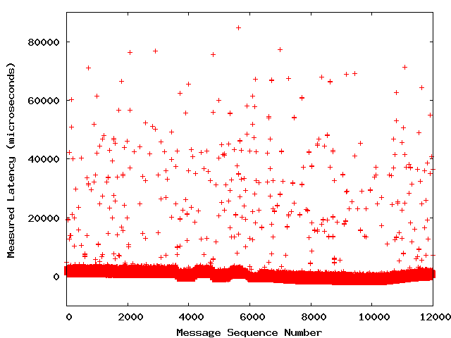
The lack of a significant change lead us to conclude that if CPU scheduling latency was the cause of the large maximum latency, then it wasn't due to CPU contention with other user time sharing processes on the machine.
This led us to try a CPU scheduling class offered by Solaris called "real time." We used the command prefix priocntl -c RT -e to request real time scheduling for all UM processes. This had a dramatic effect on the maximum latency, reducing it over 16 fold to just 5.2 ms. The plot below shows this.
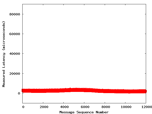
The seemingly random incidence of high-latency messages completely disappeared when UM ran with real time priority. We conclude that CPU scheduling latency was the primary cause of the large maximum latency we saw in earlier test. However, it seems that the source of CPU contention was something within the Solaris kernel since maximum user CPU priority produced no reduction in latency.
21. Measuring CPU Contention Latency
A special form of CPU scheduling latency called CPU contention latency happens when there are more runnable processes than CPUs. In effect, this separates the fixed portion of CPU scheduling latency from the variable portion. In our final round of tests, we wanted to investigate the effect of CPU contention on latency. In the preceding tests, 10 receiver processes had to contend for time on 4 physical CPUs. Note that a single multicast packet wakes up all 10 receiver process at the same time. Assuming an otherwise idle machine, 4 processes get scheduled onto CPUs immediately while 6 wait.
For this test, we ran only 3 receiver processes on the same 4-CPU machine. The results are shown in the lower line on the plot below. The upper line shows the usual 10 receiver case from above. But note that the vertical axis covers only about 1/7 the latency range of the preceding plots. The range of the vertical scale was reduced to show more detail.
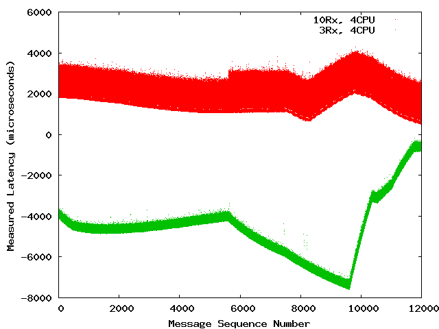
The lower band is much thinner than the upper one since there were fewer receivers than CPUs and hence no CPU contention. The difference in thickness is a good indication of how long the additional receivers in the earlier tests had to wait for a CPU to run them (the CPU contention latency). From inspection of the plot above, we'd estimate the CPU contention latency for the 10 receiver case to be about 1.5 ms.
With the magnified vertical scale of the above plot, the clock drift over the duration of the test is also apparent. This makes it easy to visualize the operation of ntpd in trying to keep the system clocks synchronized. Note that the approximately 7 ms. of clock drift during the test run significantly exceeds the measured latency for almost all of the test. Also note that the clock skew was negative for the entire 20-minute duration of the test.
Copyright 2004 - 2023 Informatica, LLC.